Two-sided Laplace transform
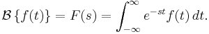
In mathematics, the two-sided Laplace transform or bilateral Laplace transform is an integral transform closely related to the Fourier transform, the Mellin transform, and the ordinary or one-sided Laplace transform. If ƒ(t) is a real or complex valued function of the real variable t defined for all real numbers, then the two-sided Laplace transform is defined by the integral
The integral is most commonly understood as an improper integral, which converges if and only if each of the integrals
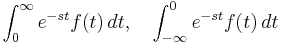
exists. There seems to be no generally accepted notation for the two-sided transform; the  used here recalls "bilateral". The two-sided transform used by some authors is
In pure mathematics the argument t can be any variable, and Laplace transforms are used to study how Differential operators transform the function.
In science and engineering applications, the argument t often represents time (in seconds), and the function ƒ(t) often represents a signal or waveform that varies with time. In these cases, the signals are transformed by filters, that work like a mathematical operator, but with a restriction. They have to be causal, which means that the output in a given time t cannot depend of input values in higher values of t.
When working with functions of time, ƒ(t) is called the time domain representation of the signal, while F(s) is called the s-domain representation. The inverse transformation then represents a synthesis of the signal as the sum of its frequency components taken over all frequencies, whereas the forward transformation represents the analysis of the signal into its frequency components.
Contents |
Relationship to other integral transforms
If u(t) is the Heaviside step function, equal to zero when t is less than zero, to one-half when t equals zero, and to one when t is greater than zero, then the Laplace transform  may be defined in terms of the two-sided Laplace transform by

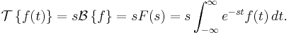
On the other hand, we also have

so either version of the Laplace transform can be defined in terms of the other.
The Mellin transform may be defined in terms of the two-sided Laplace transform by
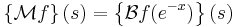
and conversely we can get the two-sided transform from the Mellin transform by

The Fourier transform may also be defined in terms of the two-sided Laplace transform; here instead of having the same image with differing originals, we have the same original but different images. We may define the Fourier transform as

Note that definitions of the Fourier transform differ, and in particular
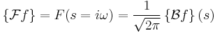
is often used instead. In terms of the Fourier transform, we may also obtain the two-sided Laplace transform, as
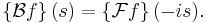
The Fourier transform is normally defined so that it exists for real values; the above definition defines the image in a strip  which may not include the real axis.
The moment-generating function of a continuous probability density function ƒ(x) can be expressed as  .
.
Properties
It has basically the same properties of the unilateral transform with an important difference
| Time domain | unilateral-'s' domain | bilateral-'s' domain | |
|---|---|---|---|
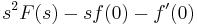
| Differentiation |  |
 |
 |
| Second Differentiation |  |
 |
 |
To use the bilateral transform is equivalent to assume null initial conditions. Therefore it is more suitable than the unilateral for calculating transfer functions from the differential equations, or when looking for an easy particular solution.
Causality
Bilateral transforms don't respect causality. They make sense when applied over generic functions but when working with functions of time (signals) unilateral transforms are preferred.
See also
- Causal filter
- Acausal system
- Causal system
- Sinc filter - ideal sinc filter (aka rectangular filter) is acausal and has an infinite delay.
References
- LePage, Wilbur R., Complex Variables and the Laplace Transform for Engineers, Dover Publications, 1980
- van der Pol, Balthasar, and Bremmer, H., Operational Calculus Based on the Two-Sided Laplace Integral, Chelsea Pub. Co., 3rd edition, 1987